An algorithm’s complexity is a metric that characterizes its performance. This article will explore the O(log n) time complexity of algorithms in detail: what it is, when it occurs, and how it helps solve problems optimally.
Main types of algorithm complexity
Before examining the main types of algorithms, it’s worth defining the concept of their time complexity. Despite its name, this metric doesn’t indicate a specific program execution time, expressed in milliseconds, for example. Rather, it estimates the number of operations performed by the algorithm for different input data sizes (denoted by the letter n).
Types of algorithm complexity:
- constant, O(1). In this case, the execution time does not depend on the size of the input data: the algorithm always executes in the same number of operations. A simple example is the function for adding two numbers:
def add_numbers(a, b):
return a + b- Linear, O(n). The execution time increases proportionally to the input data size; that is, it grows linearly: if the size increases fivefold, the execution time also increases fivefold. A classic example is finding the minimum value:
def get_min_item(arr):

    min = arr[0]

    for i in range(1, len(arr)):

        if min > arr[i]:

            min = arr[i]

return min- Logarithmic, O(log n). These algorithms reduce the amount of data to be processed at each iteration. The running time of logarithmic algorithms grows slowly relative to the input data size, so they are considered efficient. An example is binary search in a sorted array, where the number of elements to be processed is halved at each iteration. Binary search will be discussed in more detail below.
- Linear-logarithmic, O(n log n). Occurs when an algorithm combines enumeration of all elements with reduction of their number at each iteration, such as in the merge sort algorithm. In terms of efficiency, such programs range between linear and quadratic complexity.
- Quadratic, O(n²). The running time depends on the square of the input data size; some sorting algorithms, such as bubble sort, have quadratic complexity:
def bubble_sort(arr):

    n = len(arr)

    for i in range(n):

        for j in range(0, n-i-1):

            if arr[j] > arr[j+1]:

                arr[j], arr[j+1] = arr[j+1], arr[j]
If the number of elements is 100, then 10,000 operations will be required to execute the program, so the efficiency of such algorithms cannot be called high.
- Factorial, O(n!). These are the least efficient algorithms: their speed drops rapidly as the input data size increases. If n = 2, the number of operations is 2, and if n = 10, the number of operations is 3,628,800. An example is the enumeration of all possible combinations of array elements:
from itertools import permutations arr = [1, 2, 3] perm = list(permutations(arr)) print(perm) #Conclusion# [(1, 2, 3), (1, 3, 2), (2, 1, 3), (2, 3, 1), (3, 1, 2), (3, 2, 1)]
Big O Notation: A Tool for Performance Evaluation
Before considering Big O Notation, it is worth mentioning that in programming, there are three cases of algorithm performance: worst case, average case, and best case:
- The worst case is the scenario that requires the maximum amount of resources and time;
- The average case describes a scenario that requires a certain average amount of resources and time. Analyzing the average case is more difficult than the worst and best cases;
- The best case is a scenario in which time costs and resource consumption are minimal.
Big O Notation is a tool used to evaluate and analyze the performance of programming algorithms. In other words, Big O Notation describes how a program’s performance changes depending on the size of its input data. This notation allows for the comparison of algorithms in terms of their performance, selection of the optimal option, and prediction of program scalability. Big O Notation describes an upper bound on the algorithm’s execution time (the worst case): if it executes quickly in most situations, but there are cases where performance degrades, then that particular case will be described.
Big O Notation can also be used to estimate the memory complexity of an algorithm—this metric is also worth considering during design, as some programs are optimal in terms of execution time but inefficient in terms of the number of resources consumed.
Besides Big O, there are other notations:
- Big Omega – describes the lower bound on execution time (best case);
- Big Theta is needed to describe the average case.
Logarithmic Complexity O(log n): Applications and Examples
What does O(log n) mean and in what situations does it appear?
O(log n) describes situations in which the program’s execution time grows very slowly relative to the input data size (n). When might such situations arise? When the program reduces this size n at each iteration: programs with logarithmic complexity divide the original array at each iteration, for example, by a factor of 2, and continue working only with the remaining portion.
Examples of algorithms with logarithmic complexity
A classic example of such algorithms is binary search:
def binary_search(arr, number):

    left = 0

    right = len(arr) - 1

    while left <= right:

        mid = (left + right) // 2

        if arr[mid] == number:

            return mid

        elif arr[mid] < number:

            left = mid + 1

        else:

            right = mid - 1

    return -1

array = [1, 3, 5, 7, 9, 11, 13, 15]

print(binary_search(array, 9))

# conclusion: 4
Let’s look at how it works and why it has logarithmic complexity:
- There is a sorted array containing 8 elements (n = 8): [1, 3, 5, 7, 9, 11, 13, 15]. You need to find the element with the value 9.
- Next, the search boundaries are specified: the indices of the first element of the array are 0 and len(arr) – 1.
- Finding the middle index (mid = (left + right) // 2). In this case, mid = (0 + 7) // 2. This results in mid = 3, where 3 is the index of value 7.
- The obtained value (in the code, it is arr[mid]) is compared with the desired one: 7 < 9, which means that the desired element is located in the right part of the array; the left one can be ignored.
- The value of the left search boundary changes: left = mid + 1; now the index of the element on this boundary is 4 (the right boundary remains the same).
- New mid = (4 + 7) // 2 = 5; the element with index 5 is 11. 11 > 9, which means the element we are looking for is located on the left side.
- At this step, the left boundary of the search is the array element with index 4, and the right boundary changes: right = mid – 1 = 5 – 1 = 4. 4 is the index of the sought-after value 9, and it has been found. The search completed in 3 iterations.
Thus, binary search reduces the array by a factor of 2 at each iteration; it discards the part of the array in which the sought value cannot be, therefore it has logarithmic complexity.
Searching in a binary search tree works on a similar principle: it starts at the root, the search value is compared with the current one, and then there are two options:
- If the desired value is less than the current one, then the right subtree is discarded;
- If the desired value is greater than the current one, then the left subtree is discarded.
The program will continue to run until the required element is found, or until there are no more nodes to check.
Comparing O(log n) with other types of complexity
Algorithms with O(log n) complexity are second only to O(1) programs in terms of efficiency, as their speed is independent of the amount of data transferred. However, constant complexity is rare, so programs with logarithmic complexity are generally considered the most efficient.
If we compare O(log n) with other types of complexity, for example, with linear, which is third in efficiency, we can already see that the difference in the number of operations to achieve the result grows rapidly.
The difference between the different types of complexity can be clearly seen in the graph.
How to analyze and evaluate the complexity of algorithms?
Big O notation implies an asymptotic complexity estimate, which leads to several rules. First, constant factors are ignored—the size of the input data has a negligible effect on these components of the formula. For example, a notation such as O(n2+5n+3) equates to a time complexity of O(n2).
Secondly, if the expression contains a sum, the term that grows faster than the others is taken into account; for example, O(n2 + 2n) = O(n2).
The first method for assessing algorithm complexity doesn’t require the programmer to perform any serious mathematical analysis: it’s based on an analysis of the program’s structure. Let’s look at some examples.
- Below is a linear search algorithm – if the desired value is found, the loop is terminated:
def linear_search(arr, item):

    for i in arr:

        if i == item:

            return i

return FalseNow we need to consider the maximum number of operations required to complete the search. In the worst case, the search will terminate after traversing all the array elements, that is, the entire input data volume, denoted by n. The search may terminate earlier, but only the worst case is taken into account, so the complexity is O(n).
- The following function contains two blocks of code that are executed sequentially, in which case the complexity is additive:
def new_function(arr):

    for i in arr:

        print(i)

    for i in arr:

        for j in arr:

            print(i * j)
The first loop iterates through all elements of an array of n elements, meaning the complexity is linear. The second block consists of an outer and a nested loop, each of which also performs a full traversal of the array—the complexity is O(n²). Now we need to add these two results: O(n + n²). The rule takes into account the term that grows faster, meaning the final complexity is O(n²).
Estimating the complexity of recursive programs is a more difficult problem, and the master theorem or substitution method is used to solve it.
Practical examples of algorithms with different complexity
Binary search and its efficiency compared to linear search
Binary search allows you to find elements much faster than linear search, and the speed gap grows as the number of elements in the array increases. For example, if the program is given an array of 15 elements as input, linear search (O(n)) will require up to 15 operations, while binary search (O(log n)) will require about 4. If the array contains a million elements, linear search will require up to a million operations, while binary search will require about 20.
Complexity of operations in data structures
Let’s consider the complexity of basic operations in several data structures:
- An array is an optimal structure if the task requires the ability to quickly access elements by index: in this case, the complexity is O(1). However, for all operations that require iteration of values, the complexity is linear;
- Hash tables allow for efficient search, insertion, and deletion of elements by keys with complexity O(1), but in the worst case, it can become linear—O(n). Accordingly, hash tables are suitable for situations where fast data access is required;
- In a binary search tree, insertion, deletion, and search operations are performed with linear complexity, and if the tree is balanced, such as an AVL tree, then with logarithmic complexity. A binary search tree also preserves the ordering of the data;
- In linked lists, inserting and deleting elements at the beginning occurs with constant complexity, but searching and accessing by index involve iterating over all nodes, so the complexity is linear;
- In a stack, the complexity of inserting and deleting elements is constant. However, since classic stack implementations are based on the LIFO (last-in, first-out) principle, access is only possible to the element at the top, and access to arbitrary elements is limited.
Application of algorithm complexity in real-world projects
In some projects, algorithmic efficiency is crucial. This applies to all programs that must process large amounts of data without degrading performance as the workload increases, for example:
- Big Data analysis applications;
- applications that process data in real time;
- web applications and social networks that process/respond to user requests.
Frequently Asked Questions about Algorithm Complexity
How do you know if an algorithm has O(log n) complexity?
An algorithm has O(log n) time complexity if the amount of data to be processed decreases with each iteration, thereby reducing the total number of operations. A prime example is binary search—this algorithm reduces the array size by a factor of 2 with each iteration.
If the original array contains 32768 elements, the search will complete in a maximum of 15 iterations (log 32768 = 15).
Why is algorithm complexity so important in programming?
An algorithm’s complexity characterizes its efficiency and indicates to the programmer how execution time will increase with increasing input data volume. Clearly, this is crucial to ensure high program performance, as latency in real-world applications leads to a variety of problems, including a degraded user experience.
How to choose a data structure with optimal complexity?
When choosing a data structure, you can usually rely on two factors: what problem needs to be solved and what operations will be performed most often: insertion, search, deletion, and sorting of elements.
For example, if a problem requires storing elements in an ordered fashion and frequently searching for a specific value, a balanced binary search tree would be the optimal data structure in terms of complexity. If the data can be stored unordered, a hash table would be preferable.
Conclusion: The Importance of Algorithm Complexity in Programming
The time complexity of programming algorithms is undoubtedly an important metric, describing the program’s performance with varying amounts of input data. This metric should be taken into account when working on real-world projects: it allows the programmer to assess the performance of the application.
To achieve the desired performance, it is worth optimizing it, analyzing the problem to be solved, and selecting the appropriate data structure to solve it.
While this article aims to emphasize the importance of defining and analyzing algorithm complexity, focusing solely on this metric is not the best idea. After all, a programmer must also consider resource consumption, code readability, simplicity, and maintainability, and, of course, pay attention to the details of the program’s implementation. Only by considering all these factors can one choose an algorithm with a given complexity.
There are also cases where efficiency is a priority:
- working with large volumes of data;
- real-time data processing;
- systems where scalability is important.
There are also opposite situations, when efficiency is of secondary importance:
- working with small amounts of data;
- learning tasks that require a quick solution rather than one that is optimal in terms of performance;
- absence of complex calculations in the application.