Karnaugh Maps (K-Maps)

The field of digital electronics and computer systems revolves around one thing: efficiency. Whether you are designing a processor, a traffic light circuit, or an automatic door system, all of these are based on Boolean logic.

However, as circuits grow in complexity, the Boolean expressions needed to describe them become bloated and inefficient. This is where the Karnaugh Map (K-Map) steps in. A K-Map is a powerful, visual tool that simplifies Boolean algebra expressions, making circuit design faster, cheaper, and more reliable.

In this guide, we will break down exactly what a K-Map is, how it works, and why it is an essential skill for any budding engineer or computer scientist.

1. What is a Karnaugh Map?

A Karnaugh Map (or K-Map) is a graphical method used to simplify Boolean algebra expressions. Invented by Maurice Karnaugh in 1953 at Bell Labs, it serves as an alternative to the cumbersome process of algebraic minimization.

Instead of writing out long strings of Boolean equations and trying to simplify them using identities like the Distributive or De Morgan’s laws, a K-Map allows you to visualize the output of a logic function in a grid. By grouping cells containing “1s” together, you can quickly identify the simplest possible expression for your logic circuit.

Why do we need it?

Every digital circuit can be represented by a Truth Table. A truth table lists every input combination and the resulting output. While truth tables are easy to read, they are often bulky. A K-Map takes the information from a truth table and rearranges it into a systematic grid that highlights patterns, allowing us to reduce complex logic gates into a minimal set.

2. Anatomy of a K-Map

To understand a K-Map, you must first understand the Gray Code. In a K-Map, cells are arranged so that adjacent cells differ by only one bit. This is the “secret sauce” of the K-Map.

The Grids

• 2-Variable K-Map: A 2×2 grid (4 cells).
• 3-Variable K-Map: A 2×4 grid (8 cells).
• 4-Variable K-Map: A 4×4 grid (16 cells).

The rows and columns are labeled using bit transitions (e.g., 00, 01, 11, 10). Note that 11 comes before 10—this is crucial for maintaining the “one-bit change” rule.

3. Step-by-Step: How to Use a K-Map

Let’s walk through the process of simplifying a logic function using a 3-variable K-Map.

Step 1: Create the Truth Table

Suppose we have three inputs (A, B, C) and an output (Y). We fill in the truth table based on the desired logic.

Step 2: Draw the K-Map

Draw the grid and label the inputs. Place a “1” in the cell corresponding to every input combination where the output is “1” in the truth table. Place a “0” (or leave it blank) for the rest.

Step 3: Grouping the 1s

This is the most important part. You must follow these rules when circling groups of 1s:

1. Size: Groups must be a power of 2 (1, 2, 4, 8, or 16).
2. Shape: Groups must be rectangles or squares. You cannot group diagonally.
3. Maximization: Make the groups as large as possible. A group of 4 is better than two groups of 2.
4. Overlapping: Groups can overlap. This helps simplify the expression further.
5. Wrapping: The map is effectively a cylinder (or torus). The leftmost column is adjacent to the rightmost column, and the top row is adjacent to the bottom row.

Step 4: Write the Simplified Expression

For each group, look at the inputs. If an input stays the same (e.g., A is always 1) throughout the entire group, keep it. If an input changes (e.g., B goes from 0 to 1), eliminate it.

4. A Practical Example (3-Variable)

Let’s say we want to design a circuit that outputs a 1 if the binary input (A, B, C) is 3, 5, 6, or 7.

1. Truth Table Values:
   • 3 (011) -> Y=1
   • 5 (101) -> Y=1
   • 6 (110) -> Y=1
   • 7 (111) -> Y=1
2. The Grid: Place 1s in the cells labeled 011, 101, 110, and 111.

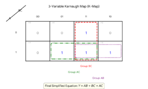
1. Grouping:
   • We can group the “1s” at 110 and 111 together. This group is “11”, meaning A=1 and B=1. C changes, so it is ignored—result: AB.
   • We can group the “1s” at 011 and 111. In this case, B=1 and C=1. A change, so it is ignored. Result: BC.
   • We can group the “1s” at 101 and 111. In this case, A=1 and C=1. B changes, so it is ignored—result: AC.
2. Final Simplified Equation: Y = AB + BC + AC.

Without the K-Map, you might have written a much more complicated equation that required twice as many logic gates!

5. Don’t Cares (X)

In many real-world design scenarios, certain input combinations will never happen. For instance, if you are working with a BCD (Binary Coded Decimal) input, the values 1010 through 1111 are impossible.

In K-Maps, we mark these as “X” (Don’t Care). The “X” can be treated as either 0 or 1, whichever helps us form a larger group. This allows for even deeper simplification.

6. Applications of K-Maps

Why do we still use K-Maps in the era of advanced software compilers?

1. Circuit Optimization

Every logic gate in a physical chip consumes electricity and takes up space on the silicon die. By reducing the number of gates required to perform a function, K-Maps directly contribute to faster, cooler, and cheaper electronic devices.

2. Embedded Systems Programming

Engineers working with microcontrollers (like Arduino or Raspberry Pi) often need to handle hardware interrupts or specific bitwise operations. K-Maps help write the most efficient C or assembly code to handle these signals.

3. Digital Logic Education

K-Maps are the standard for teaching students how to move from human-readable truth tables to machine-executable logic. It is a fundamental bridge between concept and hardware.

4. PLC Programming

Programmable Logic Controllers (PLCs) in factories use ladder logic. K-Maps help engineers consolidate complex sensor inputs into streamlined control logic, ensuring that heavy machinery operates efficiently and safely.

7. The Limitations of K-Maps

While wonderful for small-scale projects, K-Maps have a “size limit.” Once you cross into 5 or 6 variables, the maps become difficult to draw and prone to human error. For very complex systems with 10+ variables, engineers switch to computerized algorithms, such as the Quine-McCluskey Algorithm.

Conclusion

The Karnaugh Map is one of those rare “elegant” tools in engineering. It takes a tedious, manual process—algebraic reduction—and transforms it into a game of pattern recognition.

By mastering the K-Map, you aren’t just learning how to fill in grid squares; you are learning how to strip away the unnecessary and reach the absolute core of a logic function. Whether you are designing the next breakthrough gadget or just trying to pass your digital electronics course, the K-Map is an indispensable tool in your mental toolkit.

Start with a 2-variable map today, challenge yourself with a 4-variable map tomorrow, and watch as the complex world of digital logic suddenly becomes a lot more manageable.

Explore More IT Terms